Google Sheets CRM template tutorial
This Google Sheets CRM tutorial series looks at how we can build a fully, customizable, working B2B CRM to manage sales. In the first post, we started building the Google Sheets CRM, and added sheets for deals, teams, and a basic dashboard. In this post, we are going to look at improving the columns - adding sort, filter functionality, and adding dropdowns to the name and deal stage columns.
Download the Google Sheets CRM template
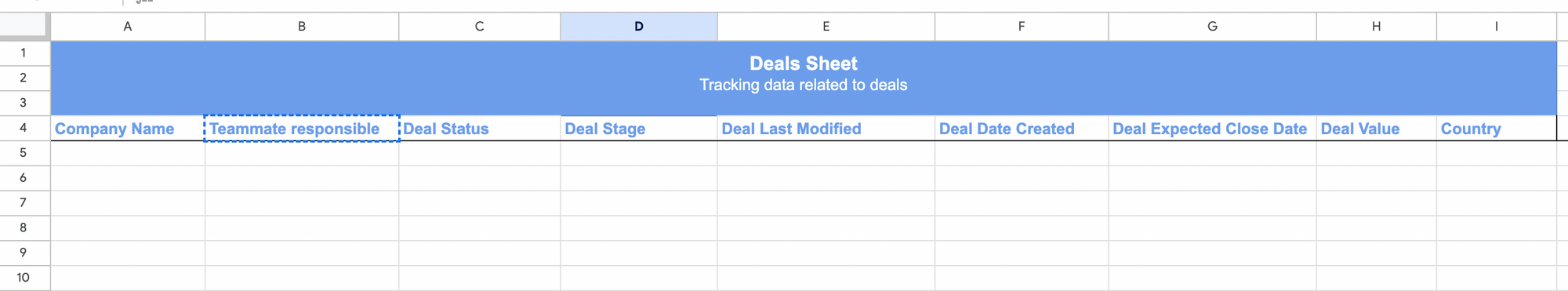
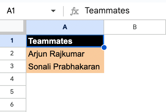
As of now we have three sheets - settings, deals and dashboard - and this is how the deals and the settings sheets looks like. If you need help creating these sheets, I would suggest starting with the first article in this series.
Customizing the Google Sheets CRM template with data validation & dropdown lists:
Ideally, to avoid errors we need to add a data validations and dropdowns. Dropdowns helps you minimize errors when you are inputting or collecting data for your CRM.
Customizing the Google Sheets CRM teammate dropdown:
Ideally the "Teammate responsible" column in the deals sheet should be a dropdown, so that anyone can click on the dropdown and select the the teammate responsible for the deal.
To start, go to the "Deals" sheets, and click on "Data", "Data validation" and then click on "+ Add rule". You will then get a box to enter the validation. Please enter the exact information as shown in the picture below:
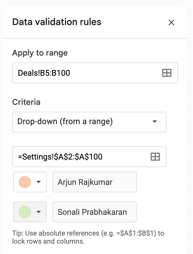
- In the "Apply to range" field, enter this: "Deals!B5:B100".
- In the Criteria field, select "Drop-down (from a range)"
- In the field below enter this, "=Settings!$A$2:$A$100"
- I have also highlighted a different colour for each person.
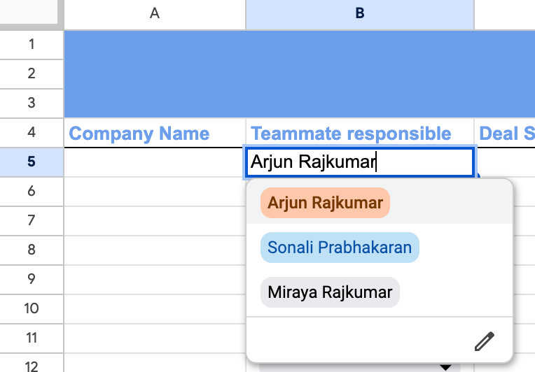
Now when we go to the "Deals" sheets, the teammate responsible will be a dropdown column with a list of all the members of the team.
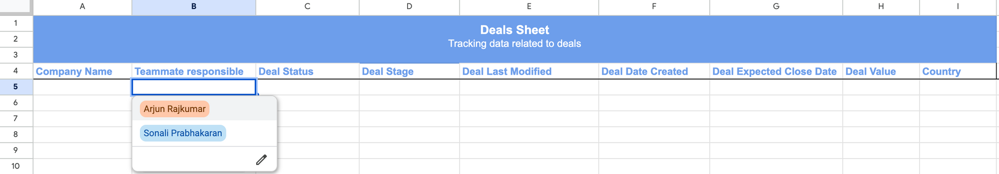
Also, we have made it so that if you update and add a new teammate, the new teammate will automatically show up in the list of selections in the dropdown.
This is great because it reduces the chance of errors, and if we want to see all the deals that one person is working on, we can easily filter that (filtering is explained later in this blog).
Customizing the "Deal Status" and "Deal Stage" dropdowns:
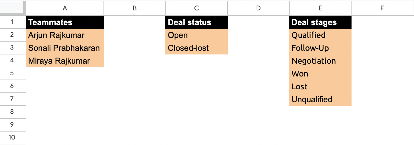
Similar to the "Teammate responsible" column we also need to add dropdowns for the deal status and the deal stage dropdown. For this, I first start by adding a new sheet called "Deal Settings", and then fill in the deal status and the deal stages columns.
The Deals stages - i.e. the milestone a potential customer has to complete on their customer journey of buying your product or service is unique to you. For now, I have added these as the defaults which you can use as is or customize according to your unique sales lifecycle.
Next, let's get these deal status and deal stages to appear in the "Deals" sheet dropdown respectively.
Adding dropdowns to 'Deal Status': Go to the "Deals" sheet and click on "+ Add rule" and fill in the following:
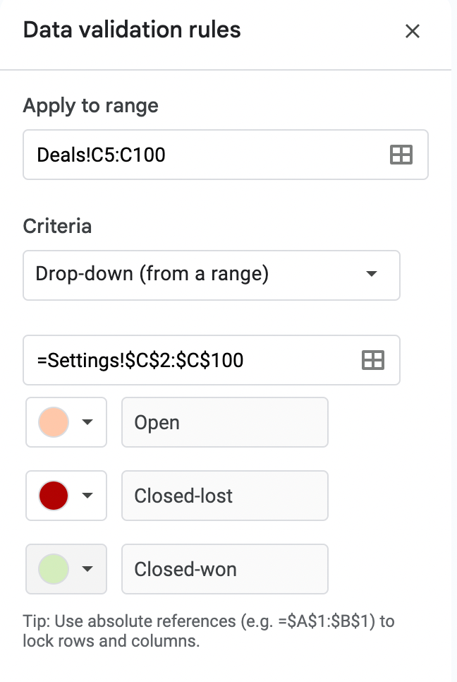
- In the "Apply to range" field, enter this: "Deals!C5:C100".
- In the Criteria field, select "Drop-down (from a range)"
- In the field below enter this, "=Settings!$C$2:$C$100"
- I have also highlighted a different colour for each deal status.
Adding dropdowns to 'Deal Stages': Go to the "Deals" sheet and click on "+ Add rule" and fill in the following:
- In the "Apply to range" field, enter this: "Deals!C5:C100".
- In the Criteria field, select "Drop-down (from a range)"
- In the field below enter this, "=Settings!$C$2:$C$100"
- I have also highlighted a different colour for each deal status.
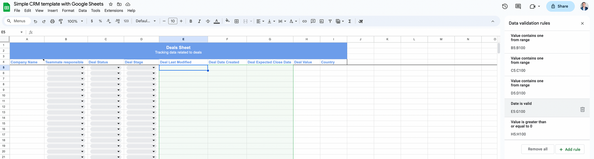
Once these three dropdowns are completed, you "deals" sheet should look something like this, where you have have dropdowns for "Teammate responsible", "Deal Status", and "Deal Stage".
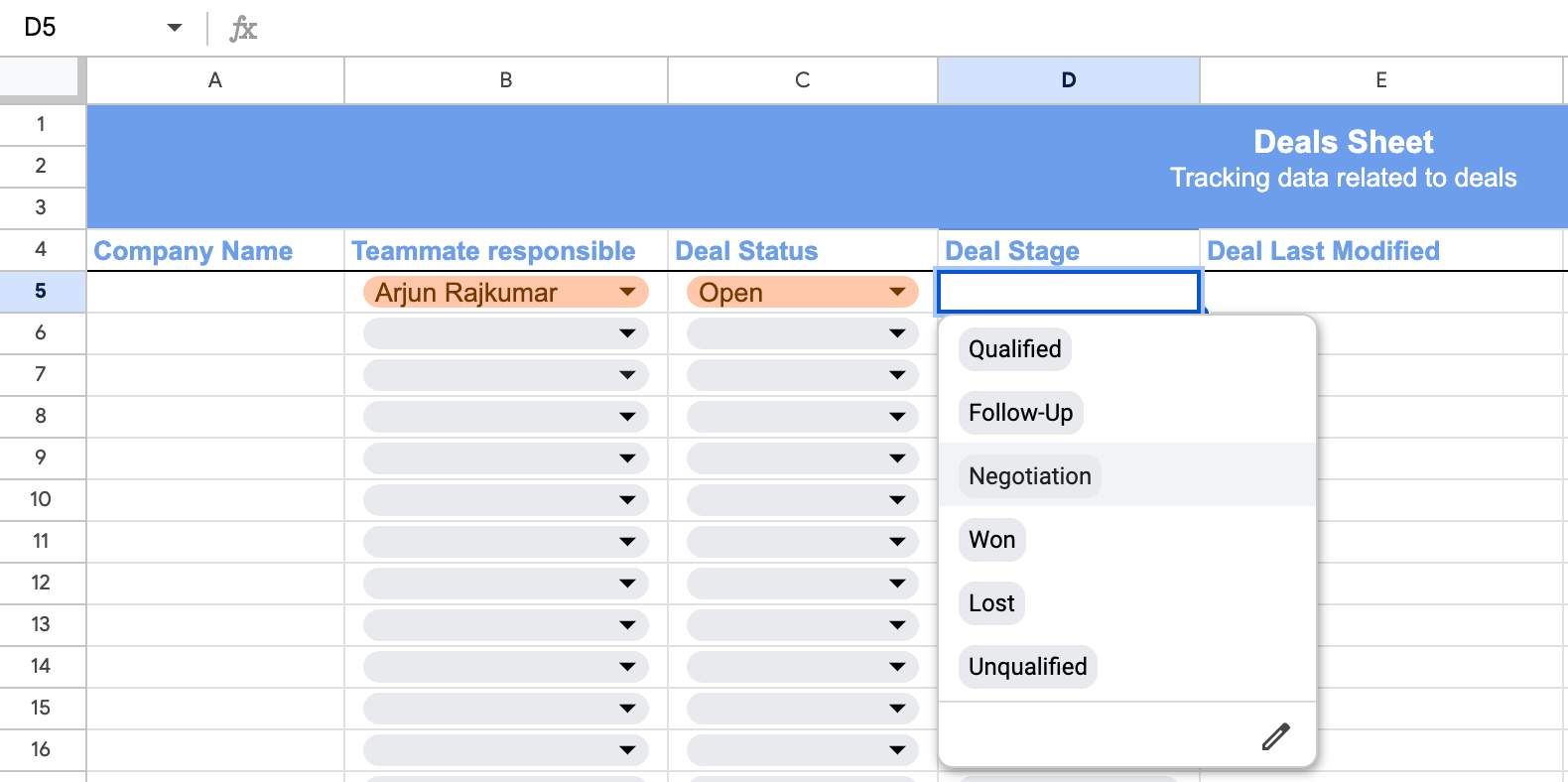
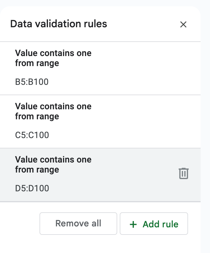
You should also see three data validations on the Deals sheet.
Adding "Data Validations" to all the other columns:
For the "Deal Last Modified", "Deal Date Created" and the "Deal Expected Close Date" column, I am ensuring that only a date can be entered in these columns. If a user tries to enter anything else other than a date, an error will appear.
I also added a note to the company name column to ask the user to enter the full company name. Later in this series, we will be adding the ability to add different customers to a company, and this company column will be updated a dropdown. For now, we are just leaving it as a note.

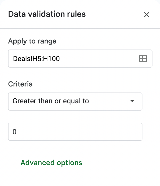
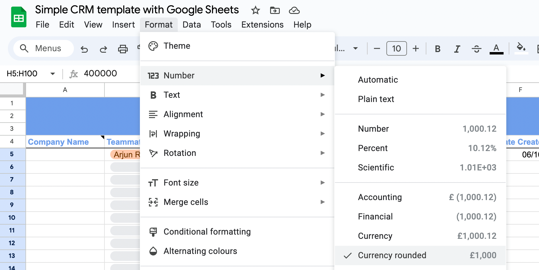
Lastly, to the "Deals value" column, I am adding a validation to ensure that only a number greater than 0 can be entered as a deal value, and I'm also formatting this to show that it is a currency.
Conditional formatting to highlight Open, Closed deals:
Next, when someone marks the "Deal Status" as "Open", I want that whole row to be orange, and when it is "Closed-lost", I want to the whole row to be red; and when it is "Closed-won", I want the whole row to be green.
First, from the Deals sheet and click on "Fill colour", and then "Conditional formatting".
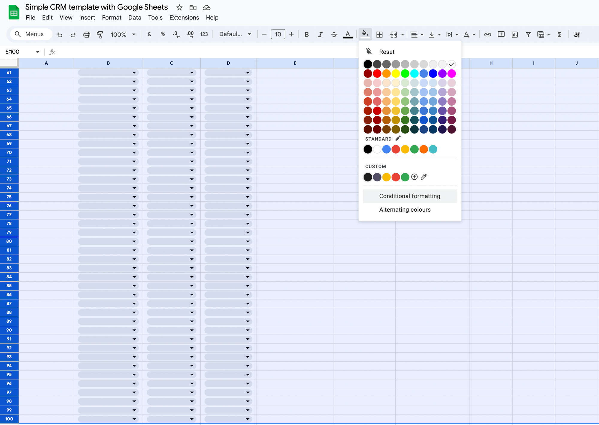
This brings up the "Conditional format rules" dialog box which we can use to colour the rows based on Deal status. We will use this dialog box to add a custom formula to colour all the cells in a row, when the "deal status" column of that row changed.
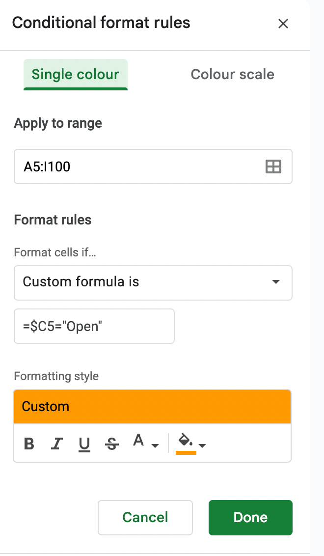
Let's start by setting the row colour to orange when the "deal status" is set to "Open". For this, I start by selecting the range i.e. A5:I100 (all the rows of the table), then selecting "Custom formula is" and setting it to =$C5="Open"
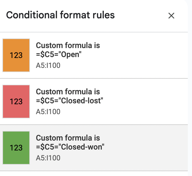
Similar, to this I also set two more conditional format rules for the "Closed-lost" and "Closed-won" deal status options. In total, I have three conditional formats applied to this page.
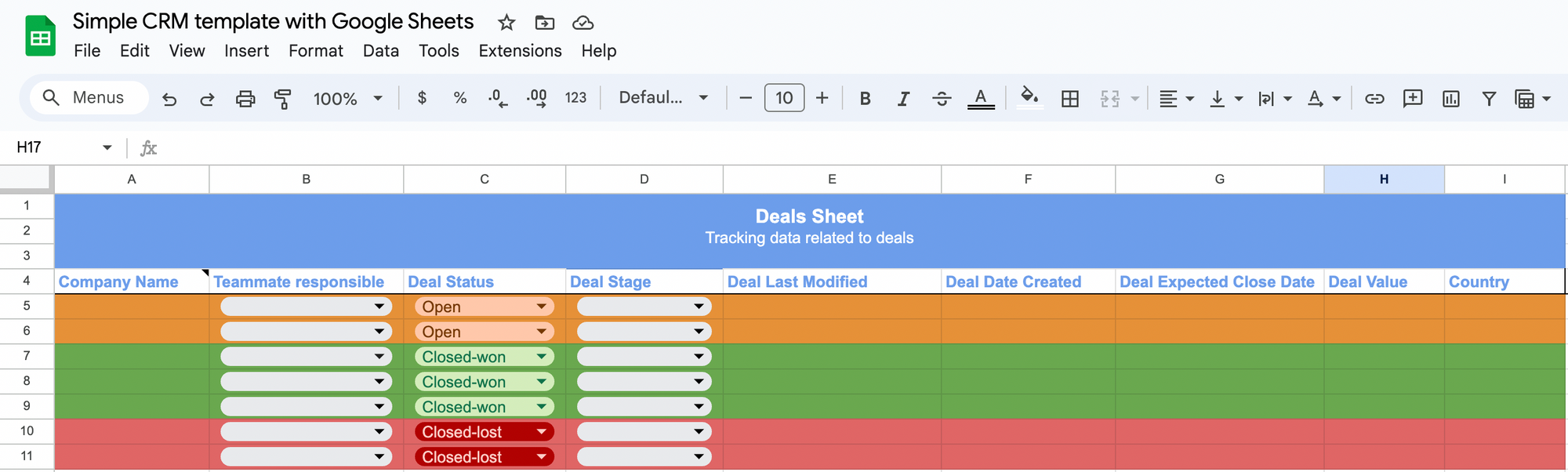
So, from now once we start entering data into the "Deals" sheet, it's colour will change depending on the status of the deal. This is great because we can quickly understand the overall progress just by looking at the sheet colours.
Sorting, filtering and cleaning CRM data in Google Sheets:
Next, lets look at how we can clean the data that is going to be entered in the CRM. First, we need to define where the headers are for the deals sheet in the CRM. We can do that by moving the freeze panes - i.e. dragging the header down manually to to the end of the 4th row.
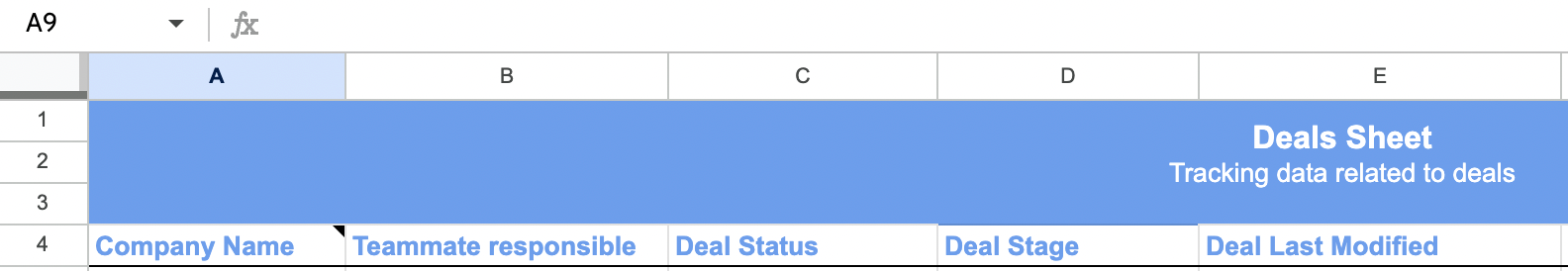
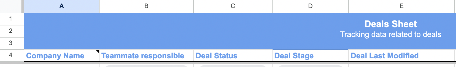
Before - After dragging the header down
This ensures that when you sort the sheet - e.g. sort by company name, the first 4 rows of the sheet remains as is, and the sorting will start only from the 5th row.
Let's add filters to make it easier to view the data. For example, you may only want to see all the deals that are in "Closed-won" state. To do this, first let's start by adding filters to the header row. Start by selecting the header row, and then the "Create a filter" icon in the menu. I have also added some dummy data to the deals sheet.
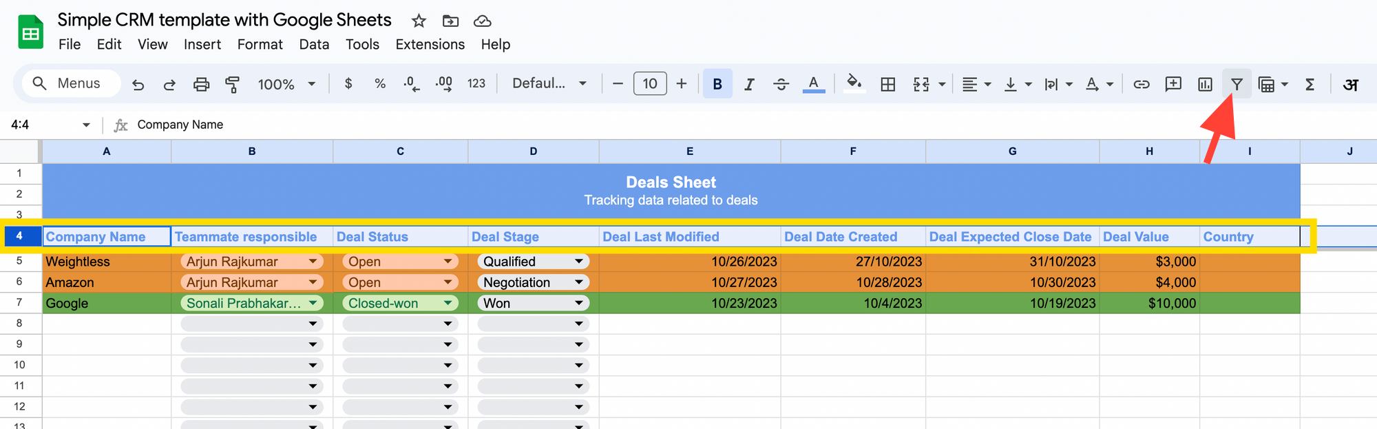
Once you create the filters, you will see the filters icon appear on the header. Now, when you click on the icons, you can select custom values to filter.

I then clicked on the "Deal status" filter, and added a condition to only show my the rows where the text contains "Closed-won".
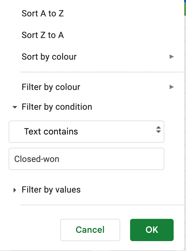
This allows me to see only the deals that have "Closed-won" status.

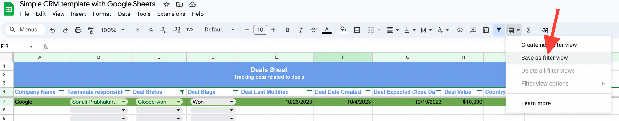
I like this view, and I am going to save this view for easy access. To do that, first click on the "Filter views" icon on top, and then on the "Save as filter view" link.
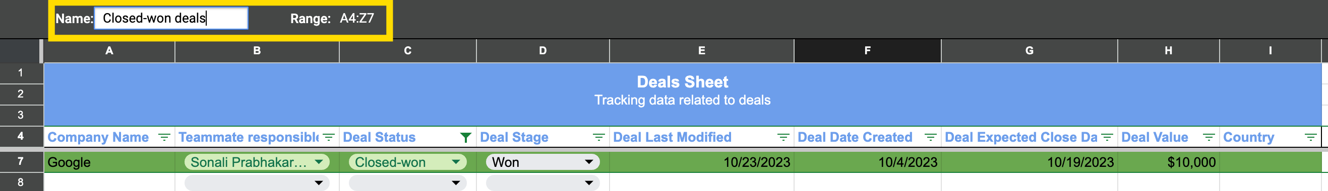
This will allow you to save this filter with a custom name of your choice. I have saved this as "Closed-won deals".
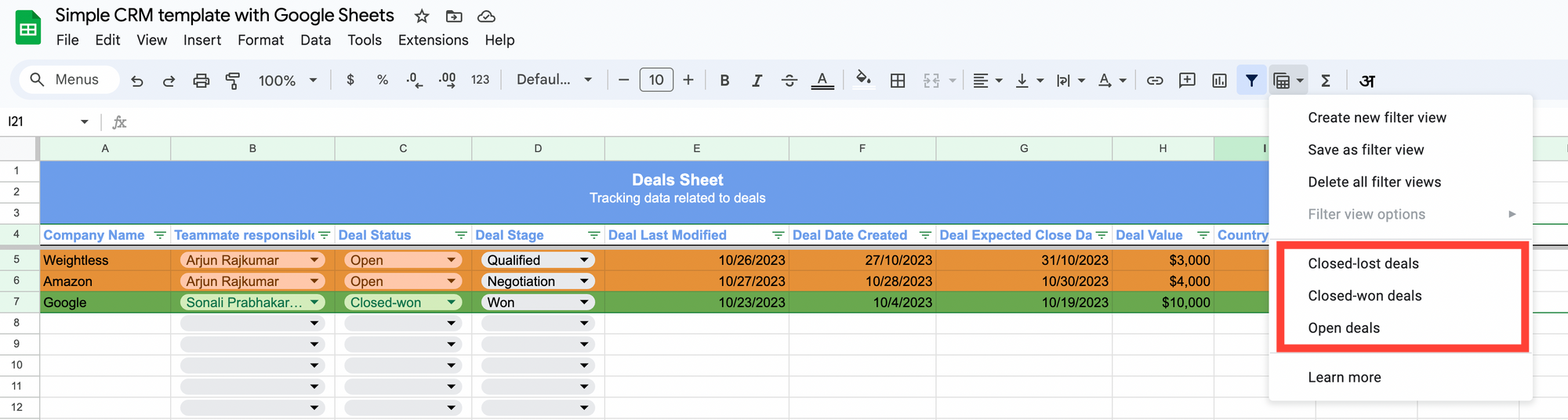
Similar, to this I also created filters for "All deals", "Closed-lost deals" and "Open deals". This way I can quickly view all filter the deals I want to see.
This completes part 2 of the google sheets CRM tutorial. In the next final article, we are going to look at a few Google Sheet CRM examples, and how you can lock certain sheets (e.g locking the "Settings" sheet), so that only you or the admins have access to those sheets to update deal stage states, or add team members etc.